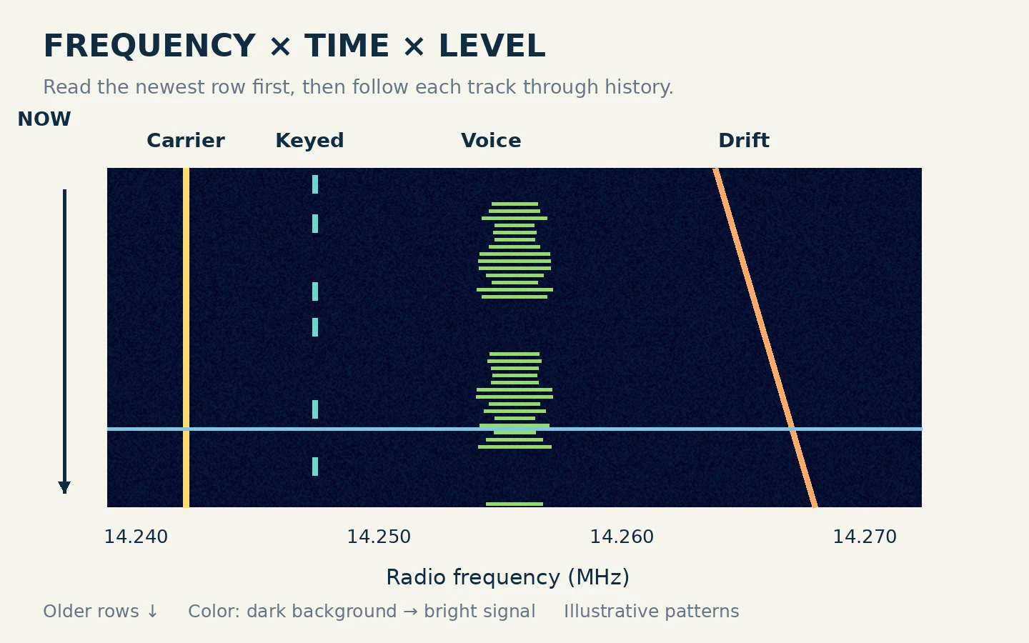
A radio waterfall shows frequency across one axis, time across the other, and received level through color or brightness. Read the frequency scale first, locate the newest row, then follow a signal through time. A narrow steady line suggests something different from a broad patch that appears only while someone speaks—but the pattern is a clue, not a positive identification.
You can learn this with a receiver or a receive-only software-defined radio, often shortened to SDR. Keep transmit controls disabled while practicing. The goal is to connect what you see with what you hear, rather than click on the brightest stripe and assume it is a usable contact.
Find Frequency, Time and the Color Scale
On a typical horizontal waterfall, frequency increases from left to right. Each new horizontal row is a spectrum taken at a particular moment. As rows accumulate, a steady signal draws a vertical track. A spectrum trace above the waterfall shows the current frequency distribution; the waterfall preserves recent history.
Check the actual scrolling direction. Many displays add new information at the top and move older rows downward, but software can use other orientations. Watch a signal appear or consult the time marks. Without knowing where “now” is, you might tune to a transmission that already ended.
Color represents the display's mapping of signal level, not a universal measurement. In one palette, dark blue may be the background and yellow a stronger signal; another may use white or red. Spectrum Lab lets the user alter this mapping through brightness, contrast and visual automatic gain control. A red line on your screen cannot be compared directly with a red line on someone else's screenshot.
Use a dark but still visible background with weak signals distinguishable from it. If everything becomes bright, reduce the display intensity or adjust its level range before concluding the whole band is occupied. This visual adjustment changes the picture; it does not by itself improve the receiver's ability to handle a strong signal.
Distinguish the Displayed Span from the Receive Filter
The span is the frequency range visible across the whole graph. The receive passband is the narrower portion the receiver processes for the audio you hear. A screen can show many signals while your receiver demodulates only one of them.
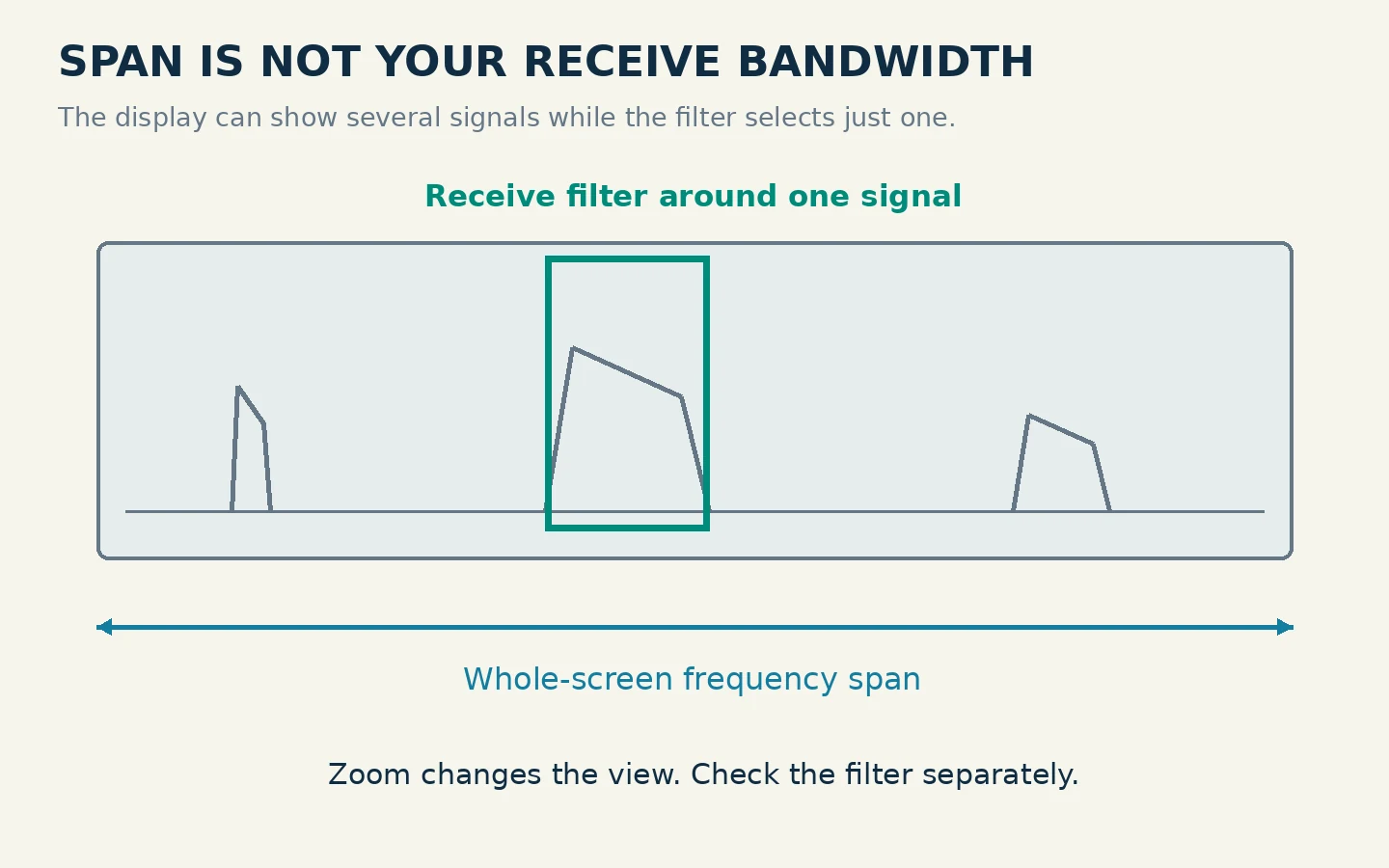
For example, a 100-kHz-wide view is useful for finding activity, but a voice signal a few kilohertz wide occupies only a small part of that view. Zooming in makes its edges easier to inspect. Zooming out shows more of the band. Neither action necessarily changes the receive filter: look for the shaded passband or filter markers to see what you are actually listening to.
The original IC-7300 manual treats scope span and receive-filter bandwidth as separate controls. Its scope is therefore a useful concrete example of the broader distinction. The exact marker colors and menu names on another radio may differ.
Before clicking a trace, also check which frequency the display uses as its tuning reference. With single sideband, or SSB, the dial marks the suppressed-carrier reference rather than the center of the visible voice energy. For upper sideband (USB), the useful passband lies above that reference; for lower sideband (LSB), it lies below it. Centering an SSB voice patch on the reference can leave the speech mistuned or partly outside the filter. The SmartSDR User Guide explicitly places the carrier reference on opposite sides of the receive passband in USB and LSB.
Check Whether the Scale Is RF or Audio
A full-band radio waterfall commonly labels actual radio frequencies in MHz or kHz. A sound-card or digital-mode waterfall may instead label audio frequencies, such as 500, 1,000 and 1,500 Hz. Those numbers are offsets inside the receiver's audio output, not separate HF band frequencies.
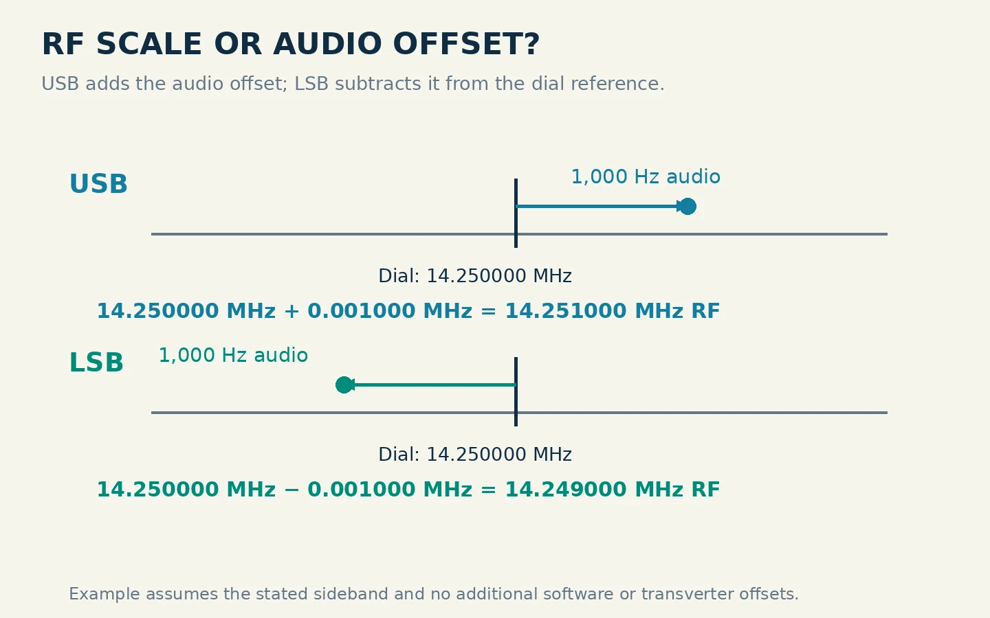
Consider a teaching example with the receiver at 14.250000 MHz in USB. An audio tone at 1,000 Hz corresponds approximately to RF at 14.251000 MHz. In LSB, the same audio offset corresponds approximately to 14.249000 MHz. The sign changes because the selected sideband changes. Other modes, software offsets and transverter configurations need their own interpretation, so establish the mode before doing this arithmetic.
This distinction matters when you write a listening note or use software that reads the radio through CAT, its computer-control interface. Record both the dial frequency and any audio offset when the application uses them separately. A waterfall label of “1500” alone is not enough to tell another operator where you were listening.
Read Common Patterns Without Over-identifying Them
In the teaching waterfall, time runs downward from the newest row. The separate shapes illustrate several useful clues:
| Visible shape | What it suggests | What to check next |
|---|---|---|
| Thin unbroken track | A steady narrow signal or carrier | Listen and see whether it remains when nearby activity stops |
| Narrow track with gaps | Keyed activity, possibly Morse code | Listen in a suitable mode; gaps alone do not prove the mode |
| Irregular wider patch | Modulated activity, such as speech | Try the appropriate demodulation mode and fine-tune |
| Sloping track | Frequency changing with time | Check whether your own tuning or reference changed |
| Brief line across much of the span | A broadband impulse or other short disturbance | Compare its timing with the sound and receiver indicators |
These are interpretations of shapes, not a signal-classification service. A narrow interference source can resemble a wanted carrier. A drifting transmitter and a changing receiver reference can both produce movement. If you change the center frequency, old and new waterfall rows may no longer share the same apparent reference unless the application compensates for that change.
Do not label another station's signal as “too wide” from a colorful screenshot alone. Display resolution, receiver settings and overload artifacts can change apparent width. Use the visible edges to guide listening and investigation, not to diagnose a transmitter you have not measured.
Adjust the Picture Before Judging the Signal
First choose a span that separates the signals you are examining. Then adjust the display's brightness or level range so the background is visible without covering the weak traces. Keep settings steady while comparing two signals.
Next consider frequency resolution and time resolution. Spectrum Lab's documentation explains that a finer frequency analysis requires a longer sample interval. A very narrow analysis can reveal close tones but respond slowly to brief events. Faster scrolling stretches events vertically; it does not make them last longer on the air.
Finally, distinguish display controls from the radio's RF controls. If your receiver shows an overflow or overload warning, follow its manual to reduce input gain, disable a preamplifier or use attenuation as appropriate. The IC-7300 manual specifically associates its OVF indication with an excessively strong input. Turning the waterfall darker would only hide the symptom.
For a practical comparison, listen to a stable signal, note the gain settings, then make one small change. If previously scattered artifacts disappear after reducing RF gain or adding appropriate attenuation, investigate receiver overload before treating every remaining stripe as a separate transmitter.
Practice One Complete Receive-only Reading
Choose an active voice signal you can hear comfortably. Begin with a moderately broad view, then narrow the span until you can distinguish that signal from its neighbors. Note the actual RF scale and where the newest data enters.
Select USB or LSB as appropriate to the signal, and fine-tune until speech sounds natural. Use the shaded receive filter to include the voice energy. Do not rely on the visual midpoint alone. Let several speech pauses pass: the irregular patch should appear and disappear in a way that relates to what you hear.
Move briefly to a nearby empty-looking place and listen. A quiet patch is evidence about your receiver at that moment, not proof that a frequency is free for transmission. Weak or intermittent stations may be absent from the recent history.
Write a short observation: UTC time, dial frequency, mode, span, receive bandwidth, and what you heard. Add “thin continuous track” or “intermittent voice-width patch” as a visual description. Repeat later with the same settings. This gives you a reproducible reading habit: scale, time, shape, passband, then sound.