A quiet HF band may reflect space weather, but it may also reflect your receiver, local noise, the frequency you chose, or the path to the station you hoped to hear. “Dead” describes what happened at a particular receiver, on a particular band and mode, at a particular place and time—not a proven worldwide band closure. No single Kp, solar-flux or sunspot number can explain one failed contact. The useful question is narrower: what changed for this path, and does evidence from the station, solar data and other received signals point to the same cause? NOAA notes that ionospheric changes can alter or even block HF transmission; that makes space weather worth testing, not the default verdict.
Define What Has Gone Quiet—and Rule Out a Station Problem
Start a short diagnostic log before looking at the solar numbers. Record the UTC period when you noticed the problem, your band or frequency and mode, your intended destination, and what you actually heard. “No replies to my calls” is different from “no signals heard,” and both differ from “signals were audible, then abruptly weakened.” Note whether the symptom concerns one desired path, several signals on one band, multiple bands, or nearly everything the receiver normally hears.
Recording UTC and comparing overlapping periods later is a practical diagnostic method, not a claim that a particular time interval proves a cause. It prevents an easy mistake: matching an event displayed for one period to listening that happened at another. If the change was sudden, record what you were hearing just before and after it. If you only discovered an apparently quiet band when you turned on the receiver, record that instead; you have not observed when any fade began.
Now look for a comparison that could challenge your first impression. Listen elsewhere on the same band and, if practical, on another band. Check a signal you would ordinarily recognize, or compare with an independent receiver’s reception of a relevant signal. A missing contact may simply mean that no one you could hear was active on that frequency. A raised noise floor suggests a different question: are signals present but buried? A broad loss of previously audible signals suggests another. None of these observations alone establishes that a whole band is closed.
Do the station check while receiving only. Confirm the intended frequency, mode, gain and other receiver settings; verify that the antenna connection is where you expect it to be. Compare the noise and signals you hear with the antenna connected and, if it is safe to do so at your station, briefly disconnected. ARRL recommends removing the antenna connection as an initial way to see whether investigated noise goes away. It says that if the noise changes only minimally, the receiver, its power supply or interference physically close to the receiver may be involved. Never transmit with the antenna disconnected.
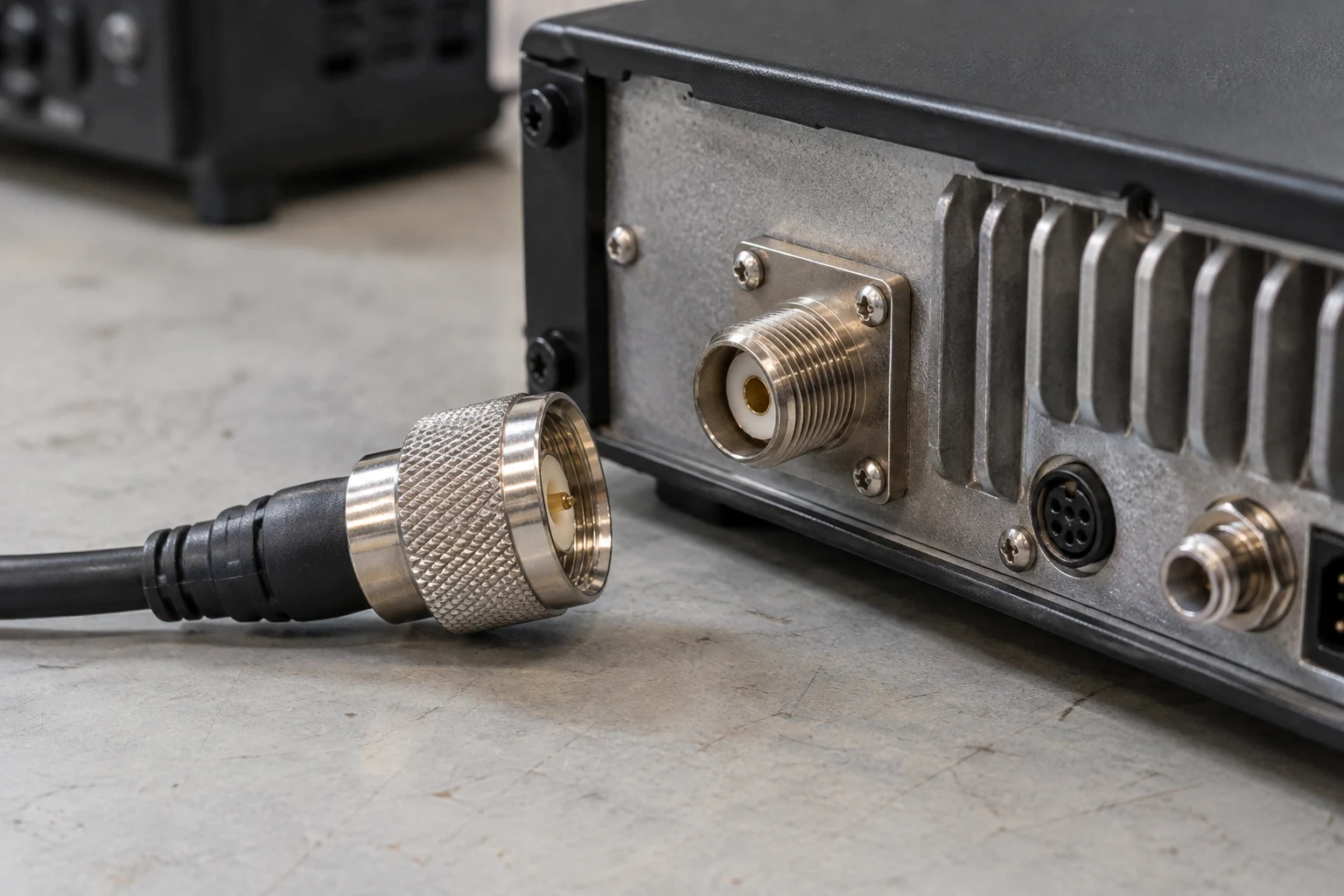
Interpret the comparison narrowly. If the noise drops markedly when you disconnect the antenna, the noise was entering through that connection; the test does not identify its source or prove a solar disturbance. If the noise scarcely changes, investigate the receiver, supply or nearby interference before blaming propagation. The test is about noise at your receiver, not whether the desired path is open. Likewise, a receiver that hears a local or otherwise easy signal has passed only that limited reception check; it has not proved that it can hear a weak, distant station on another frequency.
If you cannot make a safe antenna comparison, leave it out and use the setting checks and independent reception instead. If the station results conflict—for example, one expected signal remains clear while another disappears—keep the distinction in your log. The next steps are meant to explain the specific failure you recorded, not to replace it with a general verdict about “the bands.”
Use Sunspot and Solar-flux Figures as Background, Not a Verdict on Today
NOAA’s solar-cycle charts show observed and predicted sunspot number and F10.7-centimeter radio flux. These are useful background when you are asking what HF propagation might be like over a longer planning period. They are poor answers to the more immediate question, “Why did this signal disappear while I was listening?”
Sunspot number is commonly used in propagation prediction because, as ARRL explains, its best correlation is with monthly median ionospheric parameters. ARRL also describes 10.7-centimeter flux as a general measure of solar activity: the measured radio emission does not itself have enough energy to ionize the atmosphere. Treating a flux reading as though it were an instantaneous measure of the ionization along your route confuses the indicator with the conditions you are trying to diagnose.
The distinction matters when entering numbers into a prediction tool. A monthly or smoothed solar input helps establish the background on which a prediction is based. Replacing that context with today’s sunspot number or daily 10.7-centimeter flux may feel more precise, but ARRL warns that using daily values can introduce sizable errors into propagation-prediction outputs. A daily value is not a switch that opens one band or closes another. Nor does a steady-looking solar-cycle chart rule out a disturbance during a particular listening period.
Consider a purely hypothetical planning comparison. An operator wants to try two candidate HF frequencies to reach the same destination this month. A prediction based on its intended solar input may favor one candidate more often than the other at the planned time of day. That is a reason to try the better-looking candidate, not a reason to declare the other impossible. If the operator then hears a signal fade abruptly, updating a daily sunspot number is not, by itself, an explanation for the change. The next useful evidence is a time-relevant disturbance report and reception from a comparable path.
ARRL describes HF prediction outputs, typically including maximum usable frequency (MUF) and signal strength, as statistical values with probabilities over a monthly time frame—not absolute outcomes. In other words, a prediction helps choose where and when to listen; it does not promise that a particular station will be heard. Slow solar indicators supply that planning context. To explain an apparently new failure today, keep your recorded listening period in view and move to the faster data.
Match Fast Space-weather Indicators to the Route
Before interpreting an event display, check its observation time and status against the UTC period in your log. This is an author-designed matching step: use the data that actually overlap your symptom, and note when a display is stale, missing or marked no-data. No universal number of minutes makes every product “fresh enough.” A missing or stale display cannot establish that space weather was quiet; it leaves that part of the diagnosis untested.
NOAA separates its disturbance scales into R radio blackouts, G geomagnetic storms and S solar radiation storms. Read them as different questions about your route, not three versions of a single “bad propagation” number:
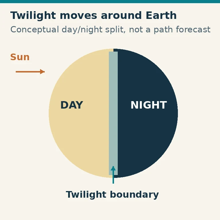
- R: Was a flare-related blackout relevant to the sunlit part of the route? NOAA places solar-flare radio blackouts on Earth’s dayside and says they are most intense where the Sun is directly overhead. Its D-region documentation explains that flare X-rays increase D-region ionization and absorption. If the portion of a route you are examining was sunlit during a time-matched R event, absorption becomes a plausible explanation for a fade. An R report by itself does not show that your particular signal crossed the affected area or failed because of it.
- G: Was geomagnetic disturbance relevant to the route? Kp belongs to the geomagnetic question, not to an immediate flare-X-ray absorption test. NOAA’s G2 Moderate example pairs Kp 6 with the possibility that HF propagation can fade at higher latitudes. That is a geographically scoped example, not a rule that Kp 6 closes HF everywhere. ARRL says a geomagnetic storm generally adds noise and weakens or disrupts ionospheric propagation for several days. That general description is not a recovery forecast for your contact.
- S: Does the route involve high latitudes affected by energetic particles? NOAA says fast-moving protons can enhance the D layer and block HF communication at high latitudes. A time-matched S event therefore deserves particular attention for a polar or high-latitude route. It should not automatically be assigned as the cause of silence on every other path.
For the R or particle-related absorption question, NOAA’s D-Region Absorption Prediction product, D-RAP, offers a more geographically useful view than an event label alone. Its global map shows a modeled highest affected frequency (HAF). NOAA defines that global HAF as the frequency suffering 1 dB of loss on a vertical path from the ground through the ionosphere and back to the ground. The product also includes an attenuation bar graph and status information. Look at the relevant part of the global map for the route and period you recorded, rather than taking a striking color anywhere on Earth as an answer about your signal.
That definition is essential to reading the map. The vertical ground–ionosphere–ground model is not your complete, oblique transmitter-to-receiver path. Its 1 dB HAF is not a universal DX cutoff or proof that every frequency beneath a color failed. The global map can support an absorption hypothesis where its modeled affected area overlaps a relevant route; it cannot, on color alone, confirm a lost contact or tell you when that contact will recover.
NOAA’s polar D-RAP maps use a different HAF definition: 10 dB of loss on a vertical round trip. Do not compare a polar-map color with a global-map color as though they represented the same attenuation. For the worked diagnosis below, use the global map and its 1 dB definition only.
NOAA says D-RAP components update continuously using one-minute GOES X-ray flux and five-minute GOES proton flux data. Those are inputs to the product, not a guarantee that the display you happen to open overlaps your own listening period. Check its shown time and status anyway. Once you have identified an event and its plausible geographical footprint, the remaining test is whether actual signals along a comparable path changed as the hypothesis suggests.
Compare a Path Prediction with Signals That Are Actually on the Air
Set up the prediction for the contact you wanted, not an unspecified “HF conditions” route. Enter the intended transmitter and receiver locations, month, time of day and candidate frequencies. The ITU’s listed HF prediction inputs also include sunspot number, transmitter power, and transmitter and receiver antenna types. If you cannot represent the actual power or antennas, note the mismatch; a generic route result is a planning approximation, not a model of your station.
Look at the tool’s basic MUF or usable-frequency output as a conditional clue. The ITU lists basic MUF among prediction outputs. If your chosen frequency looks unfavorable for that route and time, try a different candidate band or listening time when you can. Do not turn the predicted MUF into a declaration that reception above it is impossible. If a particular tool also reports a lower usable frequency (LUF) or a lower edge of a usable range, treat that as the tool’s planning estimate; the cited ITU input and output list does not establish an LUF result. If a lower-frequency candidate looks poor, connect that result to absorption only when the earlier, time- and route-relevant disturbance evidence supports the connection.
The prediction needs a reality check. Listen for a relevant beacon if one is available, or consult independent weak-signal reception observations. ARRL describes WSPR—Weak Signal Propagation Reporter—as a system designed to monitor MF and HF propagation paths. A useful comparison concerns a similar route and band during an overlapping UTC period. A signal received across an unrelated path demonstrates that some propagation was possible; it does not prove that your intended route worked.
Compare both agreements and disagreements:
- Comparable signals are present, but your desired contact is absent: revisit the station result, activity on the frequency and differences between the observed and desired paths. A working comparison path does not guarantee a reply from one particular station.
- A prediction looks favorable, but comparable signals fade or disappear during a time-matched, geographically relevant disturbance: investigate that disturbance as a leading possibility. The monthly statistical prediction has not been “disproved”; it was never a promise about that instant.
- The prediction looks unfavorable, yet relevant signals are received: use the observed signals when deciding whether to keep listening or try another candidate. Do not force the observation to fit the prediction.
- Reports are missing, stale or not comparable: leave the propagation conclusion open. Try another safe receiving comparison when one becomes available rather than treating a blank report as evidence that the route was silent.
This step also keeps the alternatives proportionate. A weak-signal report near the intended route may strengthen a path comparison, but differing frequencies, modes, endpoints or observation periods limit what it can establish. The aim is not to find one display that wins the argument. It is to ask whether the station check, the path-specific plan, the disturbance’s footprint and independently received signals tell a consistent story.
Name the Likeliest Cause—or Leave the Diagnosis Open
Invented scenario: a sudden fade on a sunlit route. An operator logs an abrupt weakening of previously audible signals on one HF frequency and mode, with the desired destination and UTC period noted. Receive-only setting and antenna checks reveal no obvious station change. A separate signal comparison establishes that the receiver can still hear something, though that alone does not validate the desired route. The operator finds an observed R event whose displayed period overlaps the logged fade, then checks whether the relevant part of the hypothetical route was sunlit. NOAA’s dayside description and its X-ray absorption mechanism make flare-related absorption a candidate.
The operator next checks the matching period and relevant area on NOAA’s global D-RAP map, remembering that its HAF represents modeled 1 dB loss on a vertical round trip—not a DX cutoff. Independent reception observations on a comparable band and route also weaken during the overlapping period. If the station check, timing, geography and comparable signals all align, flare-related absorption is the leading explanation for this fade. That verdict does not say every frequency failed, and map color does not supply a recovery time. If the independent signals remain strong, the map lacks relevant coverage, or the event period does not overlap the listening log, the solar explanation loses support; the operator should revisit the path and station comparisons.
Invented scenario: noise on a different route. Another operator hears few contacts but records a conspicuously raised noise floor, rather than a clear sudden fade. During a receive-only test, disconnecting the antenna changes that noise very little. ARRL’s guidance makes the receiver, its power supply or interference close to it reasonable possibilities. An independent receiver hears relevant signals on a comparable route and band during the operator’s logged period. Together, those observations favor a local reception problem over a claim that solar activity closed the path. The operator reconnects the antenna before any transmission; the disconnected-antenna test is never a transmitting test.
That second verdict would change if the noise dropped markedly with the antenna disconnected: the investigation would shift toward noise entering through the antenna, without identifying its source from that result alone. If independent receivers also lost comparable signals and a time-matched disturbance affected the route, a propagation cause would deserve renewed attention. Conversely, an event display with missing or nonoverlapping data cannot settle either scenario.
When checks conflict, name what remains unknown. Repeat the safe receive-only comparison, obtain a genuinely comparable signal observation, or check the event display for the logged period. The diagnostic order stays the same: describe the observed failure; test station and local-noise explanations; use slow solar figures for context; match fast R, G or S evidence to the route; then compare a path prediction with live reception. Call a solar or local cause likely only when those checks support it. Otherwise, “not yet determined” is a more useful verdict than “the HF bands are dead.”