Read an ionogram from the axes inward: check the station and observation time, identify the ordinary-wave ionospheric traces, then read their critical frequencies and virtual heights. The most useful beginner distinction is between foF2, a vertical-sounding limit, and a maximum usable frequency for a particular radio path. They are related, but they answer different questions.
An ionogram helps you choose what to investigate on HF, the high-frequency radio range. It does not tell you that a particular distant station will be audible. You can do the entire reading exercise with a web browser; no transmitting equipment is needed.
Start with the Station, Time and Axes
An ionosonde is a sounder that sends pulses upward over a range of frequencies and records returning echoes. A vertical-incidence ionogram plots the sounding frequency horizontally, normally in megahertz (MHz), and an apparent height vertically, normally in kilometers. Each cluster of echo points contributes to a trace. This is a measurement of the ionosphere above the sounder, rather than a spectrum of amateurs currently on the air.
Before interpreting a curve, find three things in the header:
- Station: where the sounder is located. A distant station may be useful for a path passing near it, but it does not measure the sky above your own antenna.
- Observation time and date: use the timestamp on the actual plot. A page labeled “latest” can still display an old image. UT or UTC is the time reference used by many services; check the date when converting to local time.
- Legend and scaling status: establish what the colors and symbols mean and whether parameter values were automatically derived or checked by a person.
The Australian Bureau of Meteorology's ionogram viewer is one usable place to practice: select a station, choose an observation, and read the displayed time. Its help page describes five-minute observations from its network. That cadence is specific to that service; do not assume every station updates at the same rate.
For a US operating decision, seek measurements relevant to the geographic region or reflection area of interest. An Australian example can teach the display, but it cannot establish today's propagation over the continental United States.
Why the Vertical Axis Says Virtual Height
The sounder measures the delay between sending a pulse and receiving its echo. Converting that delay to distance as if the pulse traveled at the speed of light throughout the journey produces a virtual height, conventionally written with a prime mark: h′. Radio waves slow in the ionosphere, so that apparent height differs from the actual height of the reflecting region.
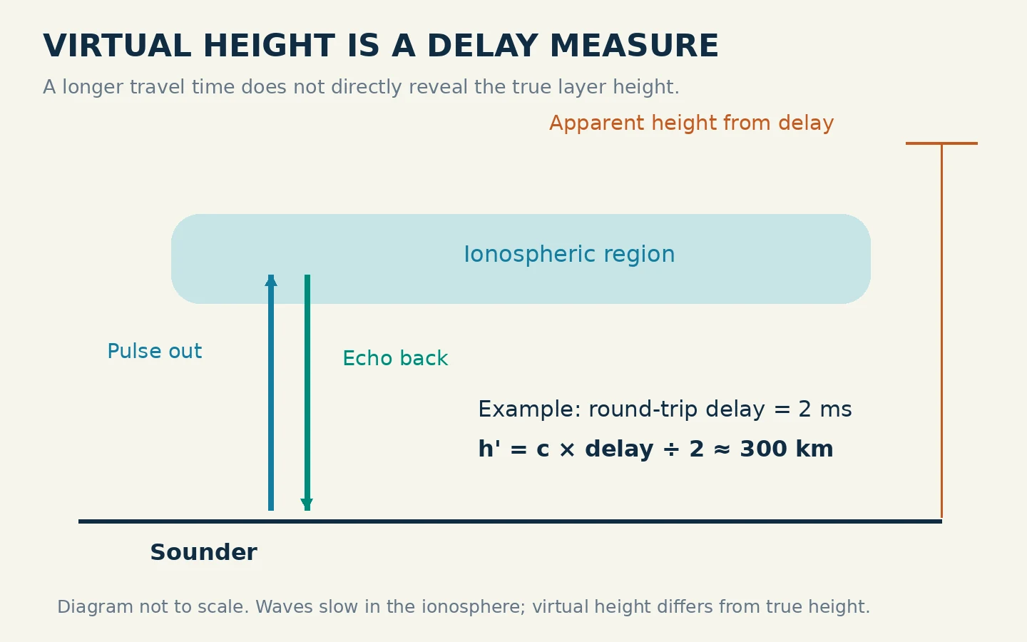
A simple teaching calculation shows the convention. Suppose the round-trip delay were 2 milliseconds. Using roughly 300,000 kilometers per second, the apparent one-way height would be 300 kilometers: multiply speed by the round-trip time, then divide by two. That calculation explains the axis; it does not determine the true height of the layer.
As the sounding frequency approaches a layer's critical frequency, the trace often bends sharply upward. Do not read that rising tail as a wall of ionosphere extending to the top of the screen. Much of the increase represents propagation delay. Likewise, h′F2 and hmF2 are different parameters: the former is a virtual-height measure, while the latter refers to the height of the F2 electron-density maximum.
Identify the Layer and the Ordinary-wave Trace
The E and F regions can return distinguishable traces. In parameter names, the letters identify the region: foE belongs to E, foF1 to F1, and foF2 to F2. Not every plot will show a tidy separate trace for every region. Start with a clean example rather than trying to force an unclear display into a textbook outline.
The lower-case o in foF2 means ordinary wave. An extraordinary-wave critical frequency is written fxF2. On a plot that shows both modes, the extraordinary trace may extend to a different frequency; that does not change which mode the “o” parameter names. These are different propagation modes in the ionized medium, not “good” and “bad” echoes. Where the display separates the modes, use its legend to locate the ordinary trace before reading foF2. Never assume that red always means ordinary or that the farthest-right colored echo must be foF2.
A sensible reading sequence is to locate the trace labeled F2, follow its ordinary-wave points toward higher frequency, and compare the upward-turning end with the horizontal frequency scale. If the service supplies an accepted foF2 value, use that together with the visible trace. Avoid inventing an extra decimal place from a coarse image.
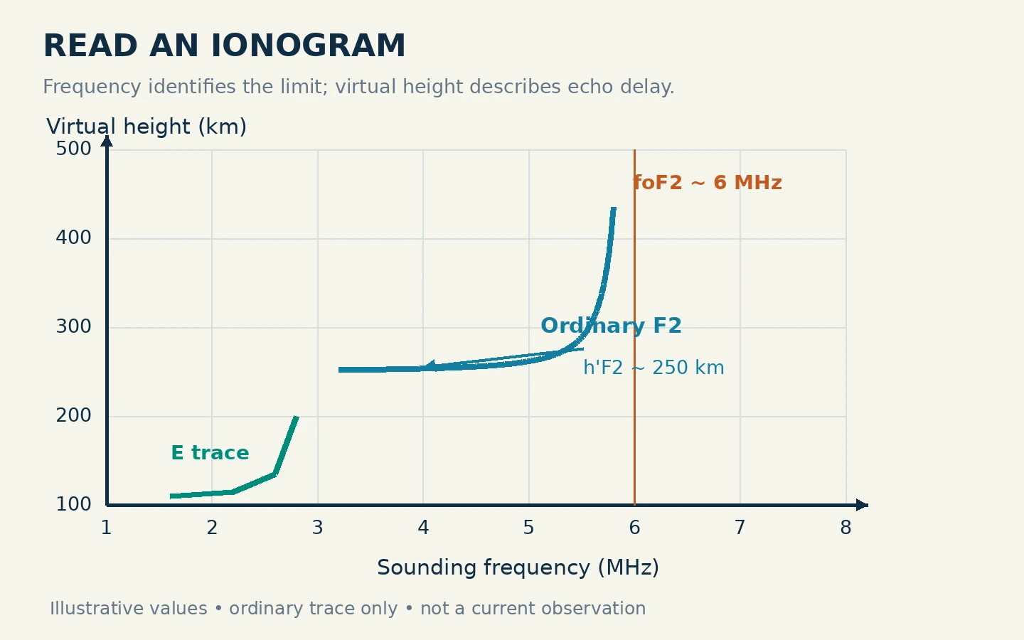
In the accompanying teaching plot, the ordinary F2 trace approaches 6 MHz and the marked minimum virtual height is about 250 kilometers. The labels are example values, not an observation from a named station. Notice that the height is read from the low part of the appropriate trace, while the critical frequency is read near its high-frequency limit. Reading both from the highest dot would mix two different measurements.
Separate foF2 from a Path MUF
foF2 is the ordinary-wave critical frequency of the highest F-region stratification. For beginner interpretation, think of it as the F2 vertical-return ceiling at the sounder's location and observation time. An oblique path travels through the ionosphere at an angle and can support a higher frequency than the corresponding vertical sounding.
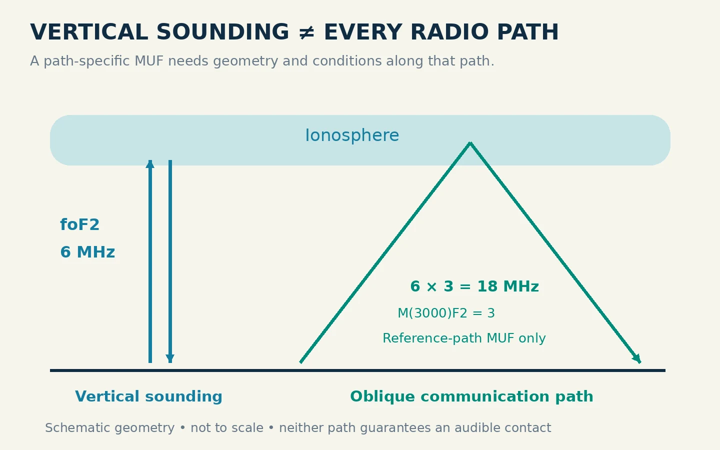
That is why “foF2 is 6 MHz, so 20 meters is closed” is an unsafe conclusion. A long-distance 20-meter path and a nearly vertical local path have different geometry. Conversely, a high path MUF does not establish that a low-power station, antenna and noise environment will produce a readable signal.
Watch for a distance inside the parameter name. MUF(3000)F2 refers to a standard 3,000-kilometer F2 path, not every possible destination. The associated M(3000)F2 is a multiplier: MUF for that reference distance divided by foF2. It is dimensionless, unlike a frequency in MHz.
For example, if a display gives foF2 = 6.0 MHz and M(3000)F2 = 3.0, their product is 18 MHz. That is the reference-path MUF in this example. It is not a recommendation to transmit at 18 MHz, and it is not a guaranteed opening to a station 3,000 kilometers from your home. The sounder location, actual path, absorption and equipment still matter.
Recognize When the Plot Is Too Uncertain
A blank area is not automatically proof that no propagation exists. First check whether the observation is current and whether the plot actually covers the frequency range you are trying to assess. A missing trace may reflect observing conditions or an incomplete return; it does not give you a reliable critical frequency to extrapolate.
The parameter fmin is the lowest frequency at which echo traces are observed. It is not the same as the lowest usable frequency of your own communication circuit. The Bureau explains that increased D-region absorption can remove low-frequency returns; a severe fadeout can even produce a blank ionogram. Check accompanying space-weather information before assigning a cause to an empty plot.
Sporadic-E parameters may appear as foEs, fbEs and h′Es. These names describe a separate E-region feature; they do not replace foF2. If the display is dominated by confusing traces, use the service's scaling notes and compare neighboring observations rather than choosing whichever number looks most promising.
Automatic numbers deserve a similar check. The Bureau distinguishes autoscaled data from partly validated data and says only its hourly foF2 values are manually checked. A plausible-looking number beside an ambiguous trace remains less useful than a clear, consistent observation.
Turn the Reading Into a Practical Listening Decision
Work through one observation and write down the station, UTC timestamp, foF2, h′F2, any reference-path MUF, and a brief quality note. Then state the question you are actually asking: nearby high-angle coverage, or a longer path toward a particular region?
For nearby coverage, compare the intended frequency with the vertical-support information while remembering that absorption can remove otherwise plausible lower-frequency options. For a longer path, consult a prediction that takes the endpoints and time into account. The Bureau's HAP charts, for example, specify a base and destination area; their meaning is more specific than a single global “band open” label.
Finally, listen on the candidate band and record what you hear. Compare a second observation later and look for a trend, keeping measurement time separate from your listening time. The useful outcome is a better-informed band choice and an honest confidence level—not a promise of contact from one curve.