Impedance describes the relationship between voltage and current at a specified frequency. In a radio system, its meaning also depends on where you are describing it: the radio output, the feed line, and the antenna feedpoint are different places with different roles. A number such as “50 ohms” is therefore not a complete description of an antenna measurement. To understand what it tells you, you need to know the frequency, the measurement location, and whether the value includes reactance.
That distinction makes antenna and feed-line readings more useful. Impedance helps explain why a load may reflect some of the signal traveling along a line, why a tuner can give the radio a favorable reading without changing the antenna-side line, and why a measurement at one frequency does not settle what happens at another.
Opposition to RF Current Is More Than Resistance
Analog Devices defines impedance, represented by Z, as opposition to electrical flow, measured in ohms. It also expresses impedance as voltage divided by current. In a DC system, impedance and resistance are the same: resistance is the voltage across an element divided by the current through it.
The RF case needs a broader idea because radio signals are alternating rather than DC. Analog Devices notes that, in AC systems, capacitance and inductance make frequency-dependent contributions called reactance. Voltage and current are still central to the impedance relationship, but they depend on frequency. Resistance alone therefore cannot always describe how an antenna system behaves at an operating frequency.
An ohm reading can answer different questions depending on its context. “What impedance does the antenna present at its feedpoint?” concerns the load at the antenna. “What is the feed line’s characteristic impedance?” concerns the line that connects it to the station. Neither question is answered fully by seeing an isolated “50 Ω” on a display or specification. Analog Devices distinguishes a transmission line’s characteristic impedance from the complex input impedance of its load; ARRL notes that an antenna’s impedance changes with the frequency fed to it.
A useful mental model is to treat impedance as a description of an electrical relationship under stated conditions, not as a permanent resistance label attached to an object. If the frequency changes, the antenna value may change. If the location changes from the antenna feedpoint to the station end of the feed line, you are asking about a different interface. Those are reasons to preserve the context around a reading, even before deciding whether it indicates a good match.
How to Read R + Jx
Keysight describes a complex impedance as having a real part, resistance R, and an imaginary part, reactance X. It gives two ways to express the same impedance: rectangular form, R + jX, or a magnitude and phase angle. The j marks the reactive part; it is not another unit or a second impedance to add after the measurement. Both R and X are expressed in ohms.
The sign of X carries information that a single positive ohm figure cannot. Rohde & Schwarz identifies positive reactance as inductive behavior and negative reactance as capacitive behavior. Zero reactance means the particular reading has no reactive part. Thus, “R is 50 Ω” does not, by itself, establish that the whole impedance is a purely resistive 50 Ω. You still need to know X.
Consider this arithmetic teaching example, not a measured antenna. Suppose a hypothetical antenna feedpoint reads 50 + j25 Ω at 14 MHz, and the line reference for comparison is 50 Ω. The resistance is 50 Ω, but the positive 25 Ω reactance indicates inductive behavior. Now suppose the reading at that same hypothetical feedpoint and frequency were 50 − j25 Ω against the same reference. Its resistance is still 50 Ω, while the negative reactance indicates capacitive behavior. The change of sign matters even though neither example changes the resistance figure.
Arithmetic applied to these invented values gives each impedance a magnitude of about 56 Ω: √(50² + 25²) ≈ 55.9 Ω. Their phase angles are about +27° and −27°, respectively, from arctan(25/50). These are calculations for the teaching example, not antenna measurements or figures reported by Keysight. The equal magnitudes conceal opposite reactive behavior. Conversely, reporting only “50 Ω resistance” conceals that both readings have nonzero reactance. Keysight’s rectangular and magnitude-and-phase forms retain that information in different ways.
Against the stated 50 Ω reference, neither example is 50 + j0 Ω. This is the important distinction when someone says an antenna is “50 ohms”: do they mean its resistance is 50 Ω, its impedance magnitude is 50 Ω, or its complete impedance is a resistive 50 Ω? Those are different descriptions. In the teaching example, the resistance happens to equal the reference, but the complete impedances do not.
The two forms also serve different reading habits. R + jX lets you see the resistive and reactive parts directly, including whether the reactance is inductive or capacitive. Magnitude and phase tell you the overall size and angle of the same complex value. Neither form makes the frequency or location optional: 50 + j25 Ω at the hypothetical antenna feedpoint at 14 MHz says substantially more than “about 56 ohms.”
Three Impedances in the Radio-to-antenna Chain
Picture the path as radio output → feed line → antenna feedpoint. A radio output may be designed for a specified impedance; the connecting transmission line has a characteristic impedance, Z₀; and the antenna acts as a load with a complex input impedance, ZL, at its feedpoint. Analog Devices uses separate terms for the line’s Z₀ and the load’s ZL. The line’s stated characteristic value is not a claim that whatever antenna you connect will have that same input impedance.
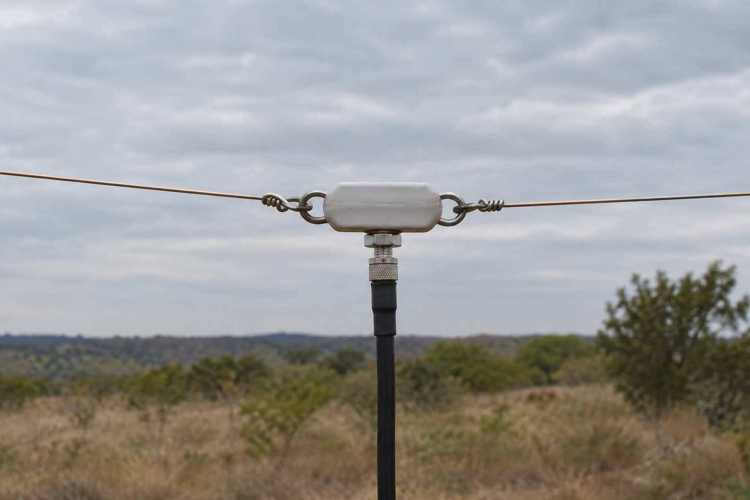
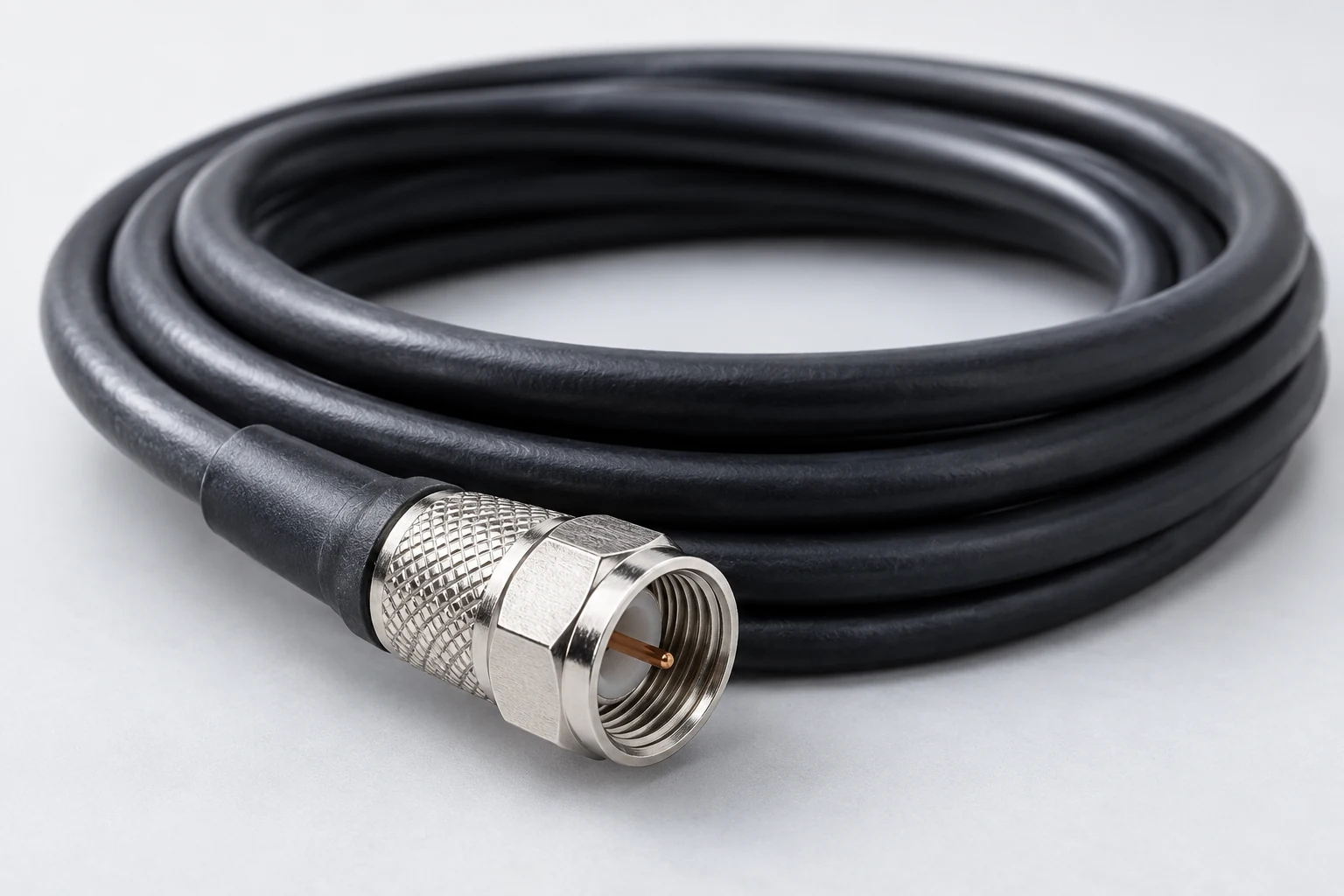
ARRL gives a familiar arrangement: radio output circuitry is usually designed for 50 Ω, with a 50 Ω coaxial feed line, and an antenna impedance of 50 Ω would match that example. This is a useful convention for interpreting many amateur-radio discussions, not a rule that every radio system or antenna must be 50 Ω. Analog Devices likewise describes 50 Ω as typical in RF engineering and explains it as a coaxial-line compromise between attenuation and power handling. It separately gives 75 Ω as a more common line choice in some broadcasting applications involving longer transmission distances and lower cable loss. That is Analog Devices’ particular example of another convention, not a property to assign to every broadcasting or amateur installation.
Keep the three values separate when reading a specification or display. A “50 Ω cable” identifies the line’s characteristic impedance. It does not force an attached antenna’s feedpoint impedance to 50 + j0 Ω. A “50 Ω radio” describes the impedance for which its output circuitry is commonly designed in ARRL’s example; it does not report the antenna’s present load. And an antenna value needs its frequency: ARRL states that every antenna’s impedance changes according to the frequency of the energy fed to it.
For an explanatory example, imagine a 50 Ω radio connected through 50 Ω coax to an antenna. If a reading at the antenna feedpoint at 14 MHz were 50 + j0 Ω, the load value would equal the line reference there. If the feedpoint reading differed at 21 MHz, the line would still be described as 50 Ω, but the load-to-line comparison would need to be made again at that frequency. This example follows from treating Z₀ and ZL as separate quantities and from ARRL’s frequency-dependent antenna description; it is not a report of a particular antenna.
This is why “Which impedance?” is a better first question than “Is it 50 ohms?” At the antenna feedpoint, you are asking what load the line meets. At the radio, you may be asking what the equipment is designed to see—or, with a tuner in between, what the tuner presents to it. The distinction prepares you to interpret a mismatch without assuming that one favorable number describes every part of the chain.
What Changes When the Load and Line Do Not Match
Analog Devices describes matching in a model that assumes the signal source is matched to the transmission line. Under that stated condition, a load is matched when its impedance equals the line’s characteristic impedance: ZL = Z₀. In that case, its model has no reflected wave at the load. If ZL ≠ Z₀, the load does not receive all the incident power. Keep the matched-source qualification attached to this explanation rather than treating it as an unconditional description of every possible source arrangement.
In the common 50 Ω comparison, the equality concerns the complete load impedance. The earlier hypothetical 50 + j25 Ω at the antenna feedpoint at 14 MHz, compared with a 50 Ω line, has 50 Ω of resistance but also 25 Ω of reactance. It is therefore not the same load value as the line reference. This is an inference from the teaching example and the load-to-line equality, not a measured reflection result.
Reflection is what standing-wave ratio, usually written SWR or VSWR, helps indicate. Rohde & Schwarz describes VSWR as a way of looking at reflection: 1:1 is the no-reflection ideal, while higher values indicate room to improve matching. Analog Devices describes return loss as the ratio of power incident on a load to power reflected back from it, used to indicate how well that load matches the network seen toward the source. These are ways to describe match quality, not alternative names for impedance’s resistive and reactive parts.
Nor is reflected power automatically the amount permanently lost as heat in a feed line. Analog Devices’ return-loss definition compares incident and reflected power; it does not define feed-line dissipation. ARRL identifies feed-line type and operating frequency as factors in how much is lost under SWR conditions. The practical question is therefore not merely “Was power reflected?” but also “What line and configuration does that reflection occur in?”
ARRL gives a concrete caution for coaxial cable under high SWR conditions, specifying greater than 3:1 in that discussion. A tuner can supply a 50 Ω match to the radio while the mismatch and high SWR persist between the tuner and antenna; ARRL warns that this situation can mean high coaxial-cable losses. The 3:1 figure belongs to that particular feed-line caution. It is not a universal transmitter-damage threshold, nor does it make every reflected watt a watt irretrievably lost.
SWR is useful precisely because it draws attention to a mismatch, but it is a summary of that aspect of the system. It does not tell you whether a load’s reactance is positive or negative, and a favorable SWR at one interface does not establish that another segment has the same condition. R + jX answers what impedance is being described; SWR and return loss address how well an impedance matches a reference at the relevant interface.
What an Antenna Tuner Matches—and What It Leaves Alone
There are two conceptually different ways to change the match being discussed. One is to change the antenna so that its feedpoint load is different at the operating frequency. The other is to leave that load as it is and use a matching device between parts of the system. ARRL calls an antenna tuner an adjustable impedance transformer that can transform the impedance of the antenna system to 50 Ω for the radio. Antenna adjustment is the load-changing alternative; it is not what a radio-side tuner accomplishes merely by showing the transceiver a low SWR.
Consider the placement first. With a tuner at the radio and a feed line continuing from that tuner to the antenna, the tuner may achieve a low SWR for the transceiver. ARRL explicitly says the SWR between the tuner and the antenna remains unchanged. Thus “the radio is matched” and “the antenna-side feed line is matched” are different statements. The radio-facing result is valuable, but it does not prove that the entire line is operating at low SWR.
How consequential that remaining line condition is cannot be read from the radio-side SWR alone. ARRL says loss associated with SWR depends on the type of feed line and the operating frequency. Its high-SWR coax example illustrates why tuner location can matter when line loss is a concern, without making a low radio-side reading meaningless or asserting that every mismatched line has the same loss.
ARRL also describes remote tuners designed to match at or near the antenna. Its favorable long-line example has a condition: the feed-line section between the remote tuner and the antenna is short. Under that condition, ARRL says the rest of the feed line back to the station can be maintained at 1:1 SWR. The segment that benefits is the long station-side line. The short tuner-to-antenna section remains on the antenna side of the matching device; placing a tuner nearby is not the same as changing the antenna’s own feedpoint impedance.
The useful question is therefore not simply “Do I have a tuner?” It is “Which interface is it matching, and which stretch of line lies on its antenna side?” For a radio-side tuner, expect its low-SWR indication to describe what the transceiver sees, not a newly matched antenna-side line. For ARRL’s conditional near-antenna example, the short antenna-side section is what allows the long return to the station to benefit. These are interpretations of placement, not an installation recipe.
Interpreting a Reading Across Frequency
An impedance display becomes more informative when you read it as a set of frequency-specific observations, rather than hunting for one favorable number. Rohde & Schwarz explains that each point on a Smith chart identifies an impedance associated with a particular frequency. A sweep therefore lets you compare readings across frequencies while retaining which point belongs to which frequency. ARRL’s observation that antenna impedance changes with frequency explains why one point cannot stand in for the whole sweep.
An R/X display makes the resistive and reactive parts explicit. A Smith chart presents those parts graphically through resistance and reactance circles; Rohde & Schwarz identifies its positive-reactance half as inductive and its negative-reactance half as capacitive. Either view can tell you something an SWR figure alone does not: whether a reading’s departure from a purely resistive reference includes positive or negative reactance. A vector network analyzer with a Smith-chart display is one instrument Rohde & Schwarz describes for examining impedance characteristics.
The chart also needs a stated reference impedance. Rohde & Schwarz notes that a Smith chart is normalized to the reference impedance selected with the equipment, such as 50 Ω or 75 Ω. A chart position or match indication should therefore be read against that selected reference, not against an assumed universal 50 Ω target. The same measured-looking number is incomplete as an interpretation if you do not know what line value it is being compared with.
The measurement plane matters too. Rohde & Schwarz emphasizes calibration at the measurement plane to compensate for cable and connector effects. In reading an antenna system, say whether the impedance is being reported at the antenna feedpoint or at the station end of a feed line. They are different reference planes; do not silently label a station-end reading as the antenna’s feedpoint value. Likewise, do not compare two displayed readings as though they describe the same interface unless their planes have been accounted for.
A workable interpretation follows this order, without requiring a Smith-chart design exercise. First, attach a frequency and measurement plane to the value—for example, “at the antenna feedpoint at 14 MHz,” rather than merely “at 14 MHz.” Check that the analyzer’s calibration corresponds to the intended plane so the intervening cables and connectors are addressed. Then read R and X against the chosen line reference, including X’s sign. Finally, use SWR or return loss as a summary of match at that plane, not as a replacement for the complex impedance reading. Rohde & Schwarz supports the frequency-point, calibration, reference, and reflection-metric distinctions; Keysight supports reading R and X as the two parts of impedance.
That leaves four questions worth carrying into any antenna or feed-line measurement: What is the full impedance value? At which frequency and plane was it obtained? Which line reference is it being compared with? And is the reading on the radio side or antenna side of any tuner? Answering those questions turns “50 ohms” or “low SWR” from an isolated reassuring number into a description of a particular part of the radio system.