To read an SWR curve, find the frequency of its lowest point, then check the SWR at the frequencies you actually plan to use. That tells you about the match to the analyzer’s selected reference impedance—not, by itself, where the antenna is resonant. Antenna-feedpoint resonance is a separate finding: the reactive part of feedpoint impedance, X, is zero. Where you connect the analyzer matters because a feedline or tuner can change what its impedance reading represents. A useful diagnosis therefore records the sweep range, operating-frequency readings, and measurement location before recommending an adjustment. The right next step may be to change a simple dipole’s length, adjust a matching network, investigate the installation, or measure closer to the feedpoint.
Find the Dip and the Usable Part of the Curve
An SWR plot shows frequency across its horizontal axis and standing-wave ratio on its vertical axis. At each frequency, the plotted SWR describes the match against the measurement system’s selected reference impedance. A 50-ohm reference is useful throughout this guide as an example; it does not mean every antenna has, or should have, a 50-ohm feedpoint impedance.
Start by reading the sweep’s lower and upper frequencies. Find the lowest plotted SWR and write down both its value and its frequency. A RigExpert analyzer, for example, can display the minimum SWR and the frequency where it found that minimum. Its plotted range is user-defined, so those displayed numbers describe the range you selected—not every frequency at which the antenna might produce a lower reading.
Next, mark the frequencies you intend to operate on. Read the curve at each end of that range and at any important frequency within it. Suppose your chosen operating range extends beyond the dip: the lowest reading may look attractive while the SWR near one edge of your range does not meet your objective. Conversely, a dip outside the range need not require an adjustment if the readings within it already meet your needs.
Decide what “acceptable” means for the particular radio and operating objective before declaring a usable window. If you draw a horizontal line at 2:1, for instance, treat it as an example threshold, not a universal pass rule. Where the curve crosses that line shows the portion of the plotted range meeting that example threshold. Then compare that portion with the frequencies you actually need. The question is not merely “How low is the dip?” but “Does the intended operating range meet the criterion I chose for this setup?”
A dip at the left or right boundary deserves another look. You have found the lowest point shown, but the curve may continue downward beyond the display. Widen the sweep to locate the dip, then narrow it around the operating range to read that range more closely. RigExpert describes its sweep mode as usable for either a broad survey or a narrow, predetermined frequency area. Record the span with the result; “1.5:1 minimum” is much less informative than “1.5:1 minimum at this frequency, on this sweep, with these readings across the intended range.”
Tell the Best Match from Feedpoint Resonance
An impedance reading can be written R + jX. R is its resistive part; X is its reactive part. At antenna-feedpoint resonance, the reactive part is zero: the capacitive and inductive contributions cancel, leaving X = 0 at the feedpoint. That definition does not require R to equal the analyzer’s reference impedance. The SWR minimum answers a different question: within the measured sweep, where is the best match to that reference? A resistive mismatch can put the minimum-SWR frequency somewhere other than X = 0.
The ARRL illustrates why “resonant” does not mean “1:1 SWR.” In its 50-ohm-line example, two purely resistive loads are 29.5 ohms and 85 ohms. Neither has a reactive component, yet each corresponds to approximately 1.7:1 SWR against that 50-ohm reference. One resistance is below 50 ohms and the other above it; zero reactance alone does not remove either mismatch.
Practical Antennas gives a separate, concrete antenna example. Its 20-meter vertical has a feedpoint impedance of 21 + j0 ohms at 14.1 MHz. The zero reactance makes 14.1 MHz its stated resonance, while its SWR there is 2.37:1. The example’s lower SWR—2.35:1—occurs instead at 14.18 MHz. The difference between those SWR figures is small, but the two frequencies answer different questions. If you reported only “the dip is at 14.18 MHz,” you would not have identified the example’s 14.1-MHz feedpoint resonance. If you reported only “it resonates at 14.1 MHz,” you would have left out the match a 50-ohm system sees there.
Those examples also prevent a common adjustment error. Moving an SWR dip and finding X = 0 are not interchangeable tuning targets. If the operating goal is to obtain a suitable match over chosen frequencies, read the SWR over those frequencies. If the goal is to locate antenna resonance, obtain R and X at the antenna feedpoint or an appropriate calibrated or de-embedded measurement plane. A low SWR reading alone cannot supply the missing X measurement; an X = 0 reading taken at an unknown point in the system cannot securely identify feedpoint resonance.
Write the two findings separately when you have both: “minimum SWR at ___” and “feedpoint X = 0 at ___.” They may coincide, but do not assume they must. If your analyzer shows only SWR, you can still make a matching decision from the curve. You simply cannot turn that curve’s lowest point into a confirmed resonance measurement.
Sweep from a Known Measurement Plane
Before connecting the analyzer, identify what you want the result to describe. For an operating-window check, list the frequencies you intend to use and the analyzer’s reference impedance. For a resonance check, plan how you will obtain R and X at the antenna feedpoint or an appropriate calibrated or de-embedded plane. Measurement plane means the location in the system that an impedance reading represents.
Use this repeatable sequence:
- Record the connection. Is the analyzer connected at the antenna feedpoint, through a short jumper, at the shack end of a feedline, or on the radio side of a tuner? Note whether the tuner is in the path.
- Set a sweep that contains the intended operating range. If you do not yet know where the dip lies, begin broadly enough to find it; use a narrower view afterward to inspect your chosen frequencies.
- Record the match, not just the headline number. Note the minimum SWR and its frequency, plus SWR at the intended frequencies and at the edges of the intended range. Record the analyzer’s reference impedance.
- Record impedance with its location. If the analyzer provides R and X, write down their frequencies and the plane they describe. Do not label a shack-end X = 0 reading “antenna resonance” without a suitable feedpoint measurement or calibration/de-embedding.
Why be so particular about the connection? The ARRL says SWR stays constant along an ideal, lossless line. But an impedance reading made through a mismatched line need not equal the impedance at its far end. Practical Antennas makes the distinction tangible: in its example, inserting a one-meter coax jumper leaves the SWR at 2.37:1, ignoring loss, while the impedance seen by the analyzer changes to 25 + j19 ohms. An operator treating that new X reading as feedpoint X would be answering the wrong question, even though the SWR appears unchanged.
A real cable adds another qualification. MFJ notes that adding cable can make observed SWR drop slightly because of resistive loss. That small drop is not, on its own, evidence that the antenna match improved. Nor should you predict a particular numerical drop from cable length alone on the strength of that observation. Record the cable arrangement and compare measurements made in like conditions.
A tuner creates a different boundary. The ARRL states that when a tuner gives the transceiver a low SWR, the SWR between tuner and antenna remains unchanged. A radio-side trace with the tuner in circuit can tell you about the match presented to the radio; it does not become the untuned antenna’s SWR curve. If you are diagnosing the antenna, identify whether the tuner was included and compare readings made at the same relevant plane. If you cannot obtain feedpoint R and X yet, report the shack-end observations honestly and make a better-plane measurement the next check rather than claiming resonance from them.
Choose an Adjustment from the Curve and Antenna Type
First decide whether the operating-window readings call for a change at all. A minimum outside your preferred frequency is not, by itself, a reason to move it when the SWR throughout your chosen range already meets your radio-specific objective. If part of that range misses the objective, the dip’s position helps you choose a direction—but only within the limits of the antenna you have.
For a full-size, length-adjustable dipole without loading or matching components, MFJ says element length mainly determines the minimum-SWR frequency. A dip below the desired frequency suggests an overlong dipole; shortening it raises the dip. A dip above the desired frequency suggests it is too short. If the dip is already in the intended range, check the SWR across the whole range before changing length simply to improve a single reading.
Make a change you can evaluate. Practical Antennas describes starting a simple half-wave dipole slightly long, then trimming or folding back the ends to bring its lowest-SWR frequency to the desired part of the band. Folding back, where practical, lets you test a shorter effective length before making an irreversible cut. Sweep again after the adjustment, using the same reference impedance and a comparable measurement plane. Check both what happened to the dip and whether the intended operating frequencies now meet your chosen objective.
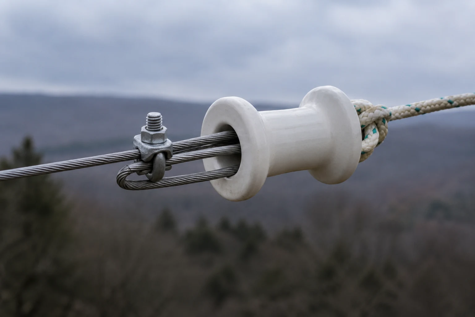
Do not make 1:1 the assumed endpoint of a length-only adjustment. Practical Antennas expressly notes that changing only the wire length may not produce exactly 1:1 SWR. Placing the dip where you want it and obtaining an acceptable operating window are related checks, not a promise that every reading can be made perfect.
Before making repeated physical changes, revisit what you know about resonance and the installation. If resonance is your goal, compare feedpoint R and X rather than chasing the SWR minimum as its substitute. If the measured dip differs from expectations, MFJ identifies ground conductivity, soil moisture, nearby wires, structures, and metal surfaces as influences worth considering. A changed installation can change the result you are trying to tune; record those conditions rather than assuming element length is the only possible cause.
Do not carry the simple dipole direction over to a loaded, trapped, matched, or otherwise complex antenna. MFJ explicitly limits its length-scaling method to full-size dipoles and verticals without loading coils, matching networks, traps, stubs, or capacitance hats. For an antenna with a built-in matching network, its recommended branch is different: begin with prescribed element settings for the target frequency, adjust the network for minimum SWR, and be prepared to revisit element and network adjustments because they interact. Recheck minimum SWR at the target frequency as the practical matching check, while also reading the rest of your intended operating range.
Finally, know when to stop adjusting the element. MFJ says large SWR changes caused by changing feedline length, repositioning the cable, or changing shield grounding should make you suspect a system problem. In that case, investigate the feedline and installation before continuing to trim according to the original curve. The first trace may not be a dependable basis for a length decision.
Work Through a Trace and Decide What It Establishes
Consider this hypothetical teaching trace, not a source measurement. An analyzer is set to a 50-ohm reference and connected at the feedpoint of a full-size, length-adjustable dipole with no loading or matching network. The sweep covers 7.00–7.30 MHz; the operator intends to use 7.08–7.22 MHz. For this example, the operator has chosen 2:1 or lower as the operating-window objective for the particular radio and use—not as a general rule.
| Frequency | Hypothetical SWR | What to mark |
|---|---|---|
| 7.05 MHz | 1.8:1 | Below the intended range |
| 7.08 MHz | About 1.47:1 | Start of intended range; feedpoint impedance is 34 + j0 ohms |
| 7.10 MHz | 1.4:1 | Lowest SWR on the sweep |
| 7.15 MHz | 1.6:1 | Within the intended range |
| 7.18 MHz | 2.0:1 | Example-threshold crossing |
| 7.22 MHz | 2.3:1 | End of intended range; above the example threshold |
First, report the dip accurately: 1.4:1 at 7.10 MHz. It is inside the intended range, but that alone does not settle the operating-window question. In this hypothetical trace, readings from 7.08 MHz through the 7.18-MHz crossing meet the chosen 2:1-or-lower objective; by 7.22 MHz, the reading does not. If the operator needs only frequencies in the portion that meets the objective, this match may already be sufficient. If operation through 7.22 MHz is necessary under the same objective, it is not sufficient across the full intended range.
Second, identify resonance independently. The stated 34 + j0-ohm feedpoint impedance at 7.08 MHz places feedpoint X = 0 there. Its approximately 1.47:1 SWR against the hypothetical 50-ohm reference is consistent with a resistive mismatch. Resonance is therefore 7.08 MHz, while the lowest SWR is at 7.10 MHz. Neither finding erases the other.
For this stated simple dipole, an operator who needs better coverage toward the high end could try a modest, reversible shortening—such as folding back the ends—then repeat the sweep and check the entire intended range. The lower-frequency dip gives a direction to test, not a guarantee that one change will satisfy the objective everywhere. If this had instead been only a shack-end SWR trace, without reliable feedpoint R and X, the justified next check would be a feedpoint or suitably calibrated/de-embedded impedance measurement; its resonance frequency would still be unknown.
Keep the conclusion bounded. Even an SWR result that satisfies the radio-side objective establishes a match at that measurement plane, not how effectively the antenna radiates. MFJ explains that its transmitted-power percentage compares forward with reflected power in the feedline; it does not state how much transmitter output ultimately performs work. Low SWR alone cannot establish radiation efficiency.